My interests lie in using machine learning to create computer models that can help further education. My undergraduate thesis is in using Bayesian Networks to learn the probability distributions of the different readings for Japanese Kanji and predict the pronunciation of a Kanji given the surrounding characters.
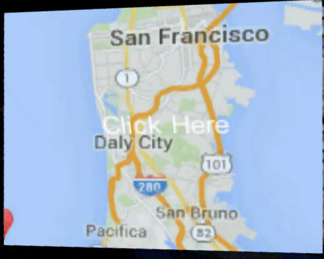
StudySubs is a WebApp for Japanese learners to upload subtitles or ebook files to study the vocabulary with Anki. The WebApp allows the user to login to track his or her progress and minimize time studying by creating flashcards for only new vocabulary for the user. StudySubs automatically extracts all Japanese from the file, tokenizes the words, conjugates each to dictionary form, tags the vocab with the pronunciation, part of speech, and English meaning. Click here to try out the WebApp.
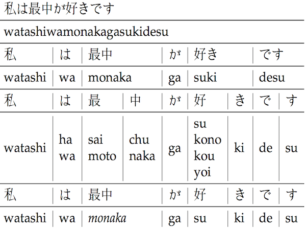
Reading Japanese is difficult for learners of the language. This is because the pronunciation of the Kanji are ambigious and can vary widely depending on the meaning and slight phonetic changes to simplify pronunciation. My undergraduate thesis explores the use of Bayesian Networks to learn the probable reading for Kanji given the context. These tractable probability distributions are then shown to the Japanese learner to help him or her understand the intuition behind Kanji readings.
Copyright © David Duffrin
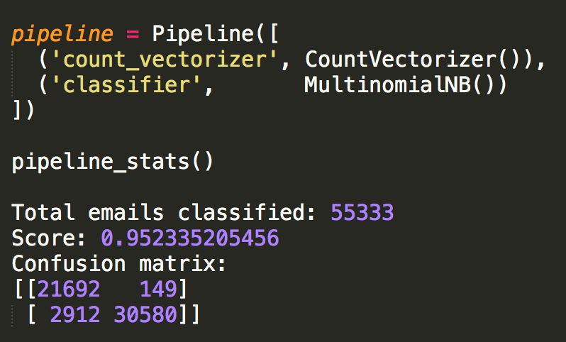
For my Optimization and Machine Learning course, I created a Naive Bayesian Spam Filter. For the technical aspects of my project, I used Python 3 with Scikit-Learn. The corpora that I collected the sample emails used for testing and training my model were the Enron emails for the “ham” data and SpamAssassin emails for the “spam” data.
I chose Naive Bayes because it is historically used for the application of spam filters. For this project I am not using as much test data as would be used in production. The classifier’s property of high bias and low variance ensures that it will converge faster and is less likely to overfit. One downside is that Naive Bayesian has a conditional independence assumption. This assumption generally holds for the features that are used in Spam Filters, however some dependence is seen in a word’s ability to be used to classify an email based on the context. An example of this is the word free. This word is usually seen in spam emails, however a friend may ask if you are free tonight. The context changes the feature from being that of spam to that of ham and so we solve for this by using bigrams to capture context.
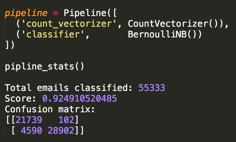
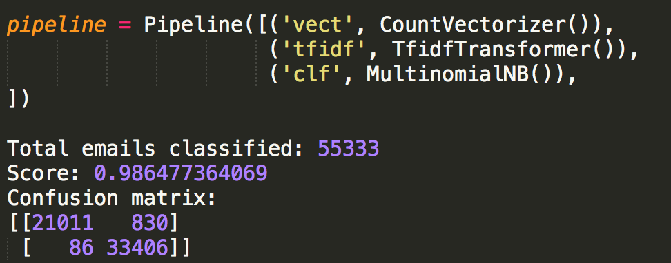
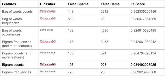
For feature selection, I looked at unigrams, bigrams, capitalization, and punctuation. Trigrams would increase accuracy but would create such a hit in performance that I felt the small gains were not worth the increased processing time. I also tried both Bernoulli and Multinomial vectorizations for the features. Bernoulli is binary with a 1 if a feature is present and 0 otherwise, while Multinomial keeps a vector with the counts for each feature. Finally I tried a tfidf transformation on the winners to see if I could improve performance. Tfidf stands for Term Frequency Inverse Document Frequency and essentially changes the counts of a Multinomial vector into percentages of the total number of features.
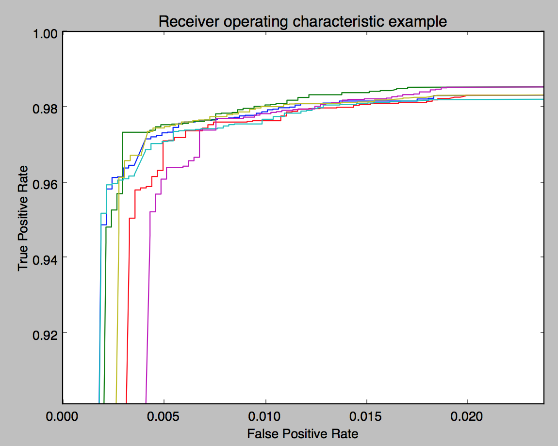
I found that the best pipeline used the Multinomial vector for unigrams and bigrams while ignoring all other features and didn’t use the transformation. This model was chosen because it minimized the false positives rate of hams being classified as spams while retaining an acceptable f1 score. A side effect of this was that false negatives are increased significantly. We can improve this model if we start to look at more features such as the sender and spelling of the email.
Spammers try to get around our filters by using a tactic called Bayesian Poisoning. Among these tactics include copying wikipedia or news articles onto the end of emails to buffer the word features and bypass the filter. There is a constant cat and mouse chase between the Spam Filter programmers and spammers to try and beat each other.
In conclusion, finding the best features is not the only way to increase the Spam Filter’s effectiveness. Other ways to improve accuracy would be to get better data and use cross validation to find better classifiers. Finally, for the top performing classifiers, the programmer must choose based on other aspects such as how fast the classifier performs.
One of my favorite homework assignments in database class was to find the "Kevin Bacon number" of given actors. I ended up downloading data from IMDB to help me with the assignment and my implementation is below.
###PostGRES #SELECT actor_id, name, 999 AS kb INTO kb_number FROM actors; #SELECT 4986 #Python3 import psycopg2 conn = psycopg2.connect("dbname=movies-duffrind user=duffrind") cur = conn.cursor() #I chose levenshtein instead of metaphore so that no matter how badly the name is misspelled, it will always return something. def find_kb(): kb_num() actor_name = input('Input actor name: ') cur.execute( """SELECT name, kb FROM kb_number WHERE levenshtein(lower(name), lower(%s)) = (SELECT min(levenshtein(lower(name),lower(%s))) FROM kb_number);""", (actor_name, actor_name)) output = cur.fetchall() for i in output: print('Actor: ',i[0],'\nKevin Bacon Number: ',i[1]) def kb_num(act = 2720, actor_list = [2720], movie_list = [], depth = 0): new_actors = [] new_movies = [] cur.execute( """SELECT kb FROM kb_number WHERE actor_id = %s;""", (act,)) num = cur.fetchall() if depth < num[0][0]: cur.execute( """UPDATE kb_number SET kb = %s WHERE actor_id = %s;""", (depth, act)) cur.execute( """SELECT movie_id FROM movies_actors WHERE actor_id = %s;""", (act,)) movies = cur.fetchall() for movie in movies: if (movie[0] not in movie_list) and (movie[0] not in new_movies): movie_list.append(movie[0]) new_movies.append(movie[0]) for movie in new_movies: cur.execute( """SELECT actor_id FROM movies_actors WHERE movie_id = %s;""", (movie,)) actors = cur.fetchall() for actor in actors: if (actor[0] not in actor_list) and (actor[0] not in new_actors): new_actors.append(actor[0]) actor_list.append(actor[0]) for actor in new_actors: kb_num(actor, actor_list, movie_list, depth + 1) find_kb()Output:
Input actor name: 50 sant
Actor: 50 Cent
Kevin Bacon Number: 103
Input actor name: kevan bekan
Actor: Sean Bean
Kevin Bacon Number: 7
Input actor name: kevin bakon
Actor: Kevin Bacon
Kevin Bacon Number: 0

Another assignment was to download the Yelp dataset and create a search for businesses by vicinity of another business.
def find_by_vicinity(business_name, category): temp = business_df[business_df['name'] == business_name].copy() lat = float(temp['latitude']) long = float(temp['longitude']) city = ''.join(temp['city']) temp = business_df[business_df['city'] == city][['name', 'longitude', 'latitude']].copy() temp['dist'] = 999.9 for i in temp.index: temp_long = temp['longitude'][i] temp_lat = temp['latitude'][i] d_long = temp_long - long d_lat = temp_lat - lat dist = d_long**2 + d_lat**2 temp['dist'][i] = dist #distance is arbitrary because I didn't sqrt temp.sort('dist') cnt = 1 for business in temp['name']: print(cnt, ': ', business) cnt += 1 find_by_vicinity(business_name, 'Automotive')Output:
1 : Flynn's E W Tire Service Center
2 : Forsythe Miniature Golf & Snacks
3 : Quaker State Construction
etc...
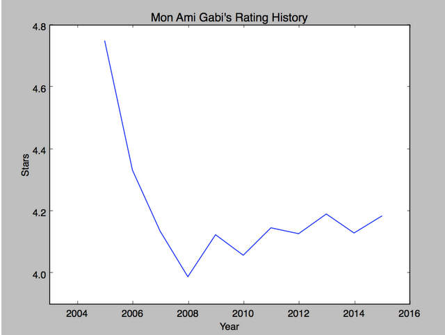
This final query uses Python and PostgreSQL to visualize the differences of a company's ratings over time. This helps us see the effects of confounding effects such as change in management as it relates to users' experience more clearly.
# Input a business’s name and it will output the history as a graph def bus_history(business_name): bus_id = business_df[business_df['name'] == business_name]['business_id'] y = list() x = [2015, 2014, 2013, 2012, 2011, 2010, 2009, 2008, 2007, 2006, 2005, 2004] y.append(np.mean(review_df[review_df['business_id'] == ''.join(bus_id)][review_df['date'] > '2015']['stars'])) y.append(np.mean(review_df[review_df['business_id'] == ''.join(bus_id)][review_df['date'] < '2015'][review_df['date'] > '2014']['stars'])) y.append(np.mean(review_df[review_df['business_id'] == ''.join(bus_id)][review_df['date'] < '2014'][review_df['date'] > '2013']['stars'])) y.append(np.mean(review_df[review_df['business_id'] == ''.join(bus_id)][review_df['date'] < '2013'][review_df['date'] > '2012']['stars'])) y.append(np.mean(review_df[review_df['business_id'] == ''.join(bus_id)][review_df['date'] < '2012'][review_df['date'] > '2011']['stars'])) y.append(np.mean(review_df[review_df['business_id'] == ''.join(bus_id)][review_df['date'] < '2011'][review_df['date'] > '2010']['stars'])) y.append(np.mean(review_df[review_df['business_id'] == ''.join(bus_id)][review_df['date'] < '2010'][review_df['date'] > '2009']['stars'])) y.append(np.mean(review_df[review_df['business_id'] == ''.join(bus_id)][review_df['date'] < '2009'][review_df['date'] > '2008']['stars'])) y.append(np.mean(review_df[review_df['business_id'] == ''.join(bus_id)][review_df['date'] < '2008'][review_df['date'] > '2007']['stars'])) y.append(np.mean(review_df[review_df['business_id'] == ''.join(bus_id)][review_df['date'] < '2007'][review_df['date'] > '2006']['stars'])) y.append(np.mean(review_df[review_df['business_id'] == ''.join(bus_id)][review_df['date'] < '2006'][review_df['date'] > '2005']['stars'])) y.append(np.mean(review_df[review_df['business_id'] == ''.join(bus_id)][review_df['date'] < '2005']['stars'])) plt.xlim([min(x)-1,max(x)+1]) plt.plot(x,y) plt.xlabel('Year') plt.ylabel('Stars') plt.title(business_name + "'s Rating History") plt.show() bus_history('Mon Ami Gabi')Output:
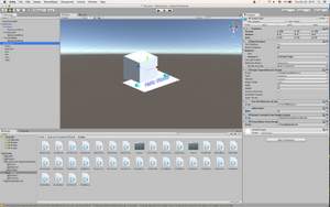
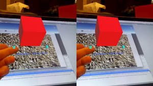
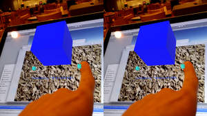
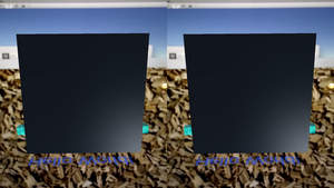
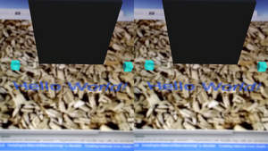
This shows my afternoon project of diving into Augmented Reality. I am interested in using this technology to interact with the user. At the time, I was unsure how to implement the Google Cardboard SDK and Vuforia at the same time, so I had to create the two camera angles myself, but now with Vuforia 5, I am able to use the ARCamera for Google Cardboard at the same time as the image recognition from Vuforia and get a more immersive experience.
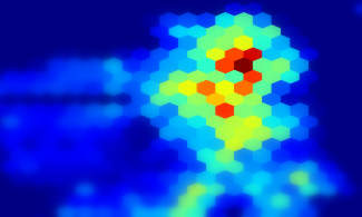
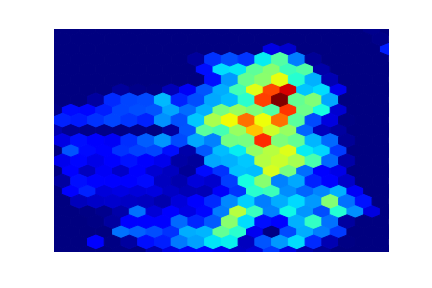
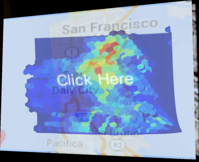
From here, I shifted my efforts from changing the color of a 3D cube, to displaying a map and using publicly available crime datasets to make 3D visualizations. I do the preprocessing in Python and then send over heightmaps, heatmaps, and other files containing height information over to be processed in C# and create the images.
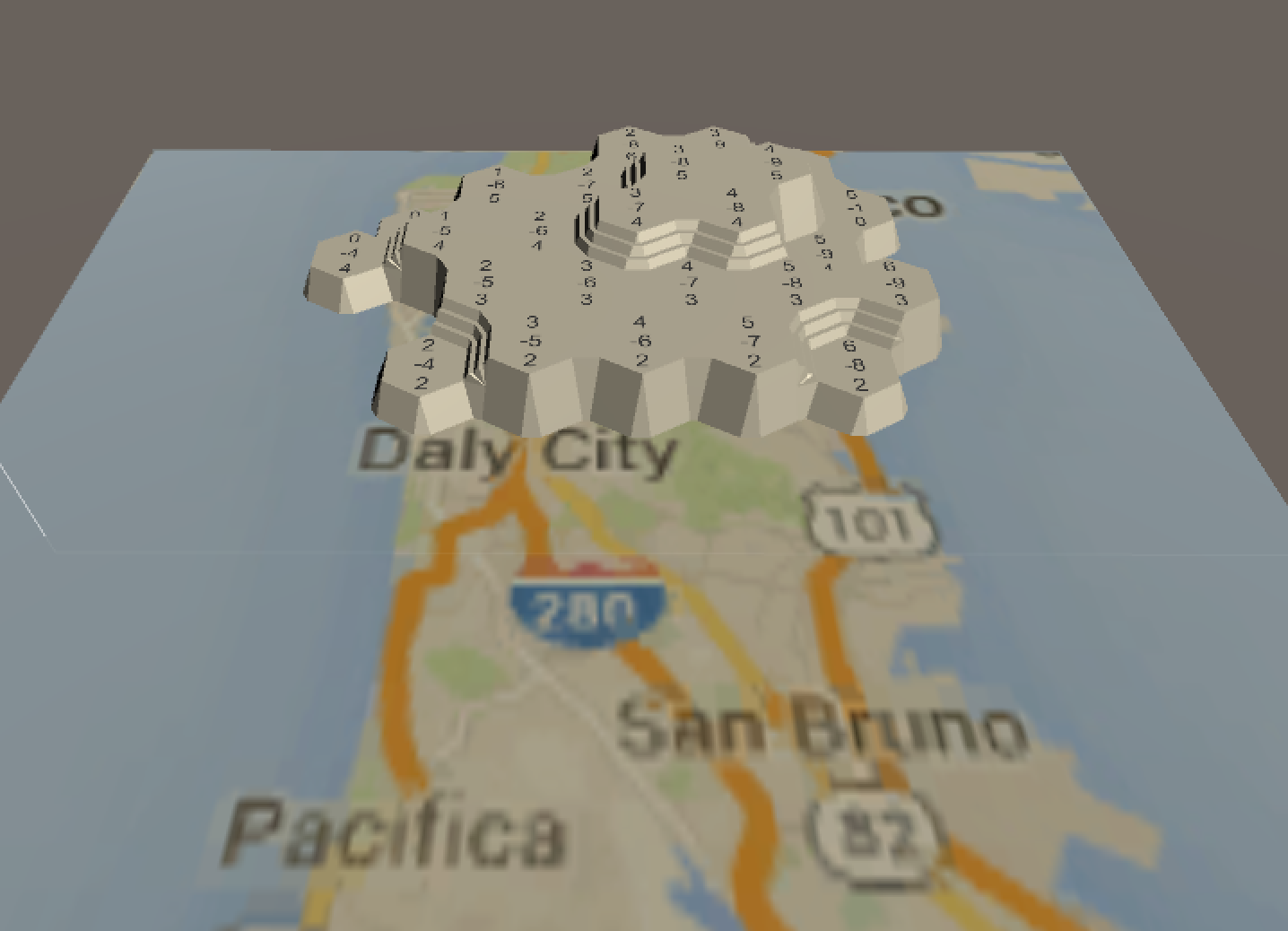
The problem here is that the 3D effect is not strong enough and the overlayed images conflict with the Google Map base. My current work is to make a text file with relative heights in Python and then creating a Procedural Mesh to create a better 3D visualization.
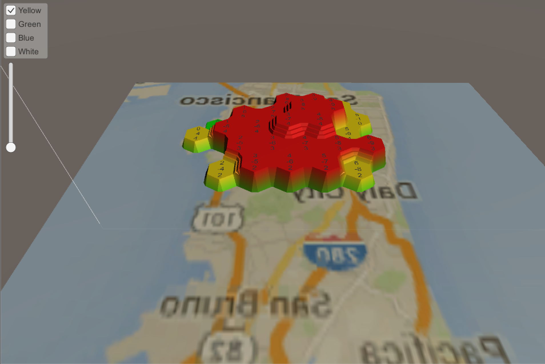
I found a tutorial on catlikecoding.com that shows how to procedurally make a map with elevation in Unity. I followed the guide and created the Google Cardboard viewable visualizations below.
Now with the visualizations in a state that I enjoy, I turned my attention to semi-automated preprocessing of the data in Python so a create file can be easily read by Unity. You can view my code on github.
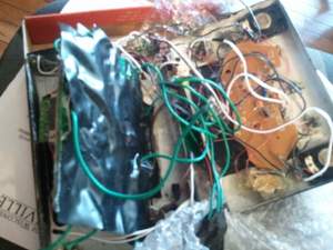
I originally got into making portable gaming consoles when I stumbled upon Palmer Luckey's website ModRetro in High School. I quickly got a part-time job and spent all of my free cash on electronics to tinker with and ultimately destroy in my path to having pocket-sized nostalgia. After many months of work, I made a custom case by vacuum forming plastic around a wooden mould, and got all the electronics to fit in and closed the case. I made the Nintendo 64 portable as seen in the picture, but had problems with the left trigger, so I opened it back up and attempted to fix the faulty button. My horrible wiring job led me to accidentally short the battery, destroying the motherboard as well as my ambition to finish.
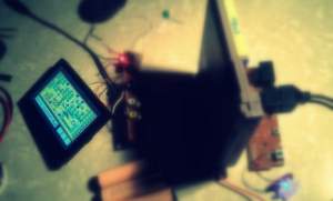
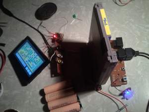
After a 4 year haitus, I decided to jump back into the portabilizing game. This time I tried a small Nintendo Entertainment System clone called a NOAC (NES On A Chip). Here is the system without the case and wired to a screen and batteries.
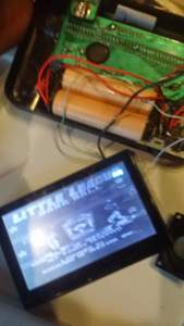
I removed more of the motherboard and tried to run the game again and was sadly shown a poorly legible black and white screen. It appears that I have taken off the video filtering and processing components so I reattached them and tried again.
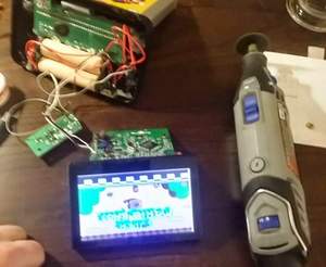
After reattaching a few components video worked great again! Now it was time to make the front of the case.
I cut the front of the case, allowing for a headphone port, volume knob, screen, buttons, power switch, charging port, and speaker slits. It is starting to resemble other portable electronics!
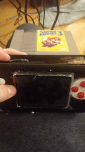
The current state of the NOAC Portable. Everything is closed and works great, but the speaker I installed is too quiet without an audio amp! Until I come back home for the holiday, I am unable to finish this up and close it for good.